Recently, I’ve taken a graduated course in Data Engineering focusing on RDBMS system, parallel data processing, etc. For some reason, I could not understand some concepts introduced in class. So, I’ve decided to take some time figuring things out by myself. In this post, I’ll discuss something about hash-based join algorithms used in RDBMS.
Let h(.) denote a hash function that produces an integer number (a.k.a, hash value) from some specific range corresponding to a given input object. h(.) is expected to satisfy some conditions as below:

$h(x) \neq h(y) \Rightarrow x \neq y ~\textrm{(1): required}$
$x = y \Rightarrow h(x) = h(y) ~\textrm{(2): required}$
$x \neq y$, then $\left\{\begin{matrix}h(x) \neq h(y) & \textrm{(3): ideal}\\ h(x) = h(y)& \textrm{(4): collision}\end{matrix}\right.$
A join of multiple relations in RDBMS is an operation that combines tuples satisfy some predicate on given attribute(s) from all relations. For simplicity, we only consider inner-join of two relations R, S here. Moreover, hash-based join algorithms are often employed for equi-join, with equal predicate, so unless stated otherwise, I’ll use join to refer to inner equi-join in this post. That’s too much for introduction, let’s dive in main points.

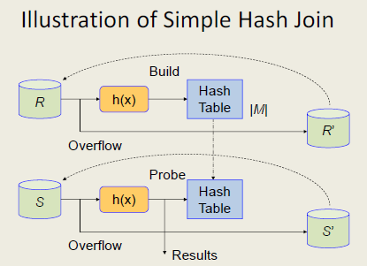
1. Simple Hash Join

Let’s assume that #|R| < #|S|, and we’re going to join R and S on attribute a. A simple hash join is simply a two-phase algorithm that:

• Build phase: Use a hash function h(.) to build a hash table for R. For example, for a tuple r in R, r will be hashed to a bucket specified by h(r.a). The main point here is that we use join attribute a to hash all tuples in R. For now, assume that the generated hash table fits into main memory.

• Probe phase: Scan all tuples of S and apply the same hash function h(.) to test if a given tuple s in S might be joined with some tuples in R. Due to property (1) of h(.), if $h(r.a) \neq h(s.a)$ then we immediately know that s should not be joined with r without comparing r.a and s.a directly. However, keep in mind that for the case $h(r.a) = h(s.a)$, we still need to check whether r.a = s.a to decide if r and s should be joined together. In probe phase, we might also write out the results to disk.
  
  The reason why hash-based algorithms might be quite efficient is that we only need to directly compare pairs (r,s) if they are hashed to the same bucket instead of doing this time-consuming task for all pairs (r,s). However, the performance of a hash-based algorithm depends on the choices of the hash function. In ideal cases, we expect that a good hash function will evenly distribute all tuples from R into let’s say n buckets, and reduce the number of collisions. Then, the expected number of tuples in each bucket is #|R|/n. This is also called load factor of the hash table. We choose hash function and n such that the load factor is a small constant. In average case, hash-based algorithm can be quite fast.

What if the hash table generated in build phase can not be fit in main memory? This situation is also known as overflow. One simple solution is iteratively run the two-phase algorithm above for |R|/|M| times, where |M| is the size of main memory. Each time, we try to fit as many tuples from R as possible into main memory. This modified algorithm is similar to block nested loop algorithm. Its main drawback is that we have to scan S for many times in probe phases. Also, it’ not easy to parallelize this simple hash join algorithm. So, smart people came up with new algorithm, called GRACE hash join!

2. GRACE Hash Join

As mentioned above, one problem with simple hash join is the overhead of scanning S for many times in case of overflow. To overcome this problem, in GRACE hash join, we use a hash function h1(.) to first split R, S into n buckets each, let’s say $R_1,...,R_n$, and $S_1,...,S_n$, respectively. This phase is called partitioning phase. The point is by dividing original relations into multiple parts, we can fit each small part into main memory. Even if it’s not the case, the overhead of scanning can still be reduced significantly. Furthermore, since the same hash function is used to partition, in the next phase (a.k.a, join phase), we only need to do join for n pairs $(R_1, S_1),...,(R_n, S_n)$. Due to the small sizes of $R_i, S_i$, compared with the original ones, the overall join cost can be reduced significantly.

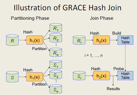
What’s more? You might notice that unlike simple hash join, GRACE hash join can be parallelized without much effort. Assume that we have n machines (processing elements), and the original relations are already partitioned into n disks in advance. Then, each disk has {R}/n and{S}/n tuples on average. Also, the selection operations on join field can be executed in parallel. In the partitioning phase, each bucket can be assigned to a machine in parallel. In other words, we can parallelize bucket decomposition in the partitioning phase. In join phase, since each machine is assigned a pair of buckets $(R_i, S_i)$, the join operation can be executed in each machine in parallel without communication with other machines. That means the join phase can be parallelized efficiently.

Let’s consider the execution cost of parallel GRACE hash join, particularly I/O cost and machine-to-machine communication cost, which are two dominating factors. It’s easy to see that in the first phase, each machine needs (|R|+|S|)/n reads and (|R|+|S|)/n writes. Also, each machine has to communicate with all of the other machines with total cost $C_{comm}$. In the join phase, no machine-to-machine communication is needed, and (|R|+|S|)/n reads for each machine. Thus, there are 3(|R|+|S|)/n I/O, plus communication cost $C_{comm}$ for each machine.

Note that, in the rough estimation above, we’ve glossed over some important factors, and only consider a rather ideal situation. What if the tuples are not distributed evenly between disks, or machines? Generally speaking, if there are data skew, the full strength and scalability of parallel system can not be achieved due to limitations of the slowest machine. In that case, the cost of skew handling is significant enough that we need to analyze carefully. Skew handling, however is beyond the scope of this small post, so I will leave it for a future post.
Also, when (|R|+|S|)/n tuples can not be fit into the main memory of each machine, then we need some techniques to deal with this situation. One common solution is double buffering, a popular technique in computer graphics that allows reading and writing from a stream continuously. Check out books or Googling for more details.
To wrap up, GRACE hash join overcomes problems in simple hash join and can be parallelized without much effort.

In this post, I briefly discussed two hash-based join algorithms: Simple Hash Join, and GRACE Hash Join from my shallow understanding. There are obviously many hash-based join algorithms out there, e.g., a popular Hybrid Hash Join, but a full discussion is beyond the scope of this blog and not my objective. I just want to nail down some basic parts which might help further understand of more sophisticated algorithms.

Happy hashing! Until next time!