It has been a while since my last post in series of machine learning for newbie. This time, we will discuss a bit on the loss functions. But what is the loss function, anyway?

0. Preliminary

Let’s get started with the problem of making prediction on new unseen data based on given training data. This problem includes both regression and classification as its specific cases. More specificially, we consider a predictive function $f: \mathcal{X} \rightarrow \mathcal{Y}$, with input (covariate, feature vector) $x \in \mathcal{X}$, and output (label) $y \in \mathcal{Y}$. For a given $x$, we try to predict its corresponding output as $f(x)$ such that $f(x)$ is as close to the true output as possible. It’s clear that we need some ways to measure how close (how good) our prediction is to the true value. That where a loss function comes in. In this post, unless stated otherwise, we consider a loss function $l: \mathcal{Y} \times \mathcal{Y} \rightarrow \mathcal{R}$ such that $l(f(x), y)$ tell you how close our prediction $f(x)$ to the true value $y$ in a quantitative manner. The problem of making prediction is simply equivalent to learning the predictive function f(x) which minimizes the expected risk:

$~~~~~~~~~~~~~~~~~~~\underset{f \in \mathcal{F}}{\mathrm{min}}\:\mathbf{E}_{P(x,y)}[l(f(x),y)]$ (*)

where $\mathcal{F}$ is our model from which we select the predictive function, P(x,y) is the underlying joint distribution of input x and output y. We will talk about model selection and how to minimize the expected risk above, e.g. empirical risk minimization (ERM) in other posts. For now, let us focus on the problem of choosing the appropriate loss function. More specifically, different types of loss functions might lead to different solutions of the minimization problem above. In other words, the loss function should be carefully selected depending on specific problems, and our purposes. From now, we will take a tour over some common loss functions and their usage.

I. Loss Functions in Regression

For simplicity, we often consider $\mathcal{Y} = \mathbf{R}$ in regression setting.

1. Squared Loss:

$~~~~~~~~~~~l(f(x),y) = (f(x) - y)^2$.
This is one of the most natural loss function we might come up with at the first place. Under this loss function, our expected solution to the minimization problem (*) is: $f(x) = \mathbf{E}[Y|X=x]$ for a given input $x$.
In other words, we will obtain the conditional mean as the solution of ordinary least squares regression with the squared loss function.

2. $\tau$-quantile loss:

$~~~~~~~~~~l(f(x),y) = (1-\tau)\mathrm{max}(f(x)-y,0) + \tau\mathrm{max}(y-f(x),0)$,
for some $\tau \in (0,1)$.
Under this loss function, our expected solution for (*) is: $\{y~|~\mathrm{Pr}(Y < y) \leq \tau \leq \mathrm{Pr}(Y \leq y)\}$. In other words, we obtain the $\tau$-quantile point of the conditional probability $P(Y|X=x)$. Especially, when $\tau = 0.5$, $l(f(x), y) = |f(x)-y|$, and the solution is the median of the conditional probability $P(Y|X=x)$.

II. Loss functions in Classification

Here we only consider the binary classification problem where $\mathcal{Y} = \{+1, -1\}$. However, the loss functions discussed here also generalize to the multiclass problems as well.

1. 0-1 loss:

In binary classification, our objective is to minimize the misclassfication error as
$~~~~~~~~~~~~~~~~~~~~~~\underset{f \in \mathcal{F}}{\mathrm{min}}~E\{\boldsymbol{1}[y \neq f(x)]\}$ (**)
where $f(x) \in \{+1, -1\}$, and $l(f(x), y) = \boldsymbol{1}[y \neq f(x)]$ is called 0-1 loss, such that:

The predictive function that minimizes the objective (**) above is called the optimal Bayes classifier:

Astute readers might notice that the discreteness of output domain ${+1, -1}$ makes our predictive function not quite comfortable to handle. So, let us consider a predictive function similar to regression case, i.e. $f: \mathcal{X} \rightarrow \mathbf{R}$, and just take the sign of this function to classify the input,

This further leads to the concept, called margin, defined as $m(x) = yf(x)$. Intuitively, a positive/negative margin means correct/wrong classification. Intuitively, the larger than 0 the margin is, the more confidence we have in our prediction. This idea is related to maximum margin classifier, where the popular Support Vector Machine (SVM) is an example.
Another problem is that while there is nothing wrong with the straightforward 0-1 loss, its non-convexity leads to difficultly in solving our optimization problem. In general, there are no guarantees about minimization with non-convex optimization functions. That’s why it is common practice in machine learning that people uses convex loss functions, whose convexities guarantees that we can find the (unique) minimum for our optimization problem, as a proxy for the 0-1 loss. See, e.g., Peter L. Bartlett, et al. Convexity, Clasification, and Risk Bounds for theoretical justification of using the convex surrogate losses. Now, let’s take a look at some common convex surrogate losses in classfication.

2. Convex surrogate losses

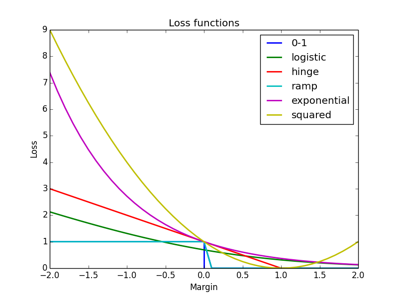
The convex surrogate losses are often defined as functions of the margin mentioned above. Intuitively, the surrogate loss should be a monotonically decreasing function, i.e., the larger the margin, the smaller the incurred loss shoud be.

* Logistic loss

$~~~~~~~~~~l(f(x), y) = log(1 + exp(-yf(x))) = log(1 + exp(-m(x)))$.
This loss function is used in Logistic regression, which actually is a classification technique despite its name. From the probabilistical perspective of logistic regression, minimizing the logistic loss is equivalent to maximizing the conditional log-likelihood log P(Y|X).

* Hinge loss

$~~~~~~~~~~l(f(x), y) = max(1-yf(x), 0) = max(1-m(x),0)$.
This loss function is used in Support Vector Machine. Since it is unbounded as the margin is getting negatively smaller, this loss function may be sensitive to outlier in the data. Its bounded variant, called Ramp loss is proposed to be more robust against outlier.
$~~~~~~~~~~l_{Ramp}(f(x), y) = min(1, max(1-yf(x),0))$.

* Exponential loss

$~~~~~~~~~~l(f(x), y) = exp(-yf(x)) = exp(-m(x))$.
This loss function is often used in Boosting algorithm, such as Adaboost. What Adaboost actually does is minimizing the exponential loss function with training data. Again, its sensitiveness to noise in data leads to many proposed robust boosting algorithms, e.g., Madaboost, Logitboost which use more robust loss functions.

$~~~~~~~~~~l_{logit}(f(x), y) = log(1+exp(-2m(x)))$.

Since a picture might worth a thousand words, let me conclude with an illustrative figure, including plots of loss functions we discussed in this long post. Until next time!

Recently, I came across a nice post on basic combinatorics. It brings back some vague memory from my middle school time when I started to learn very basic stuff related to combinations, permutations, etc. At first, I was not too excited about figuring out those formulae on my own. As time goes by, however, I’ve realized that the intuitive meanings, principles under the hood are incredibly useful and interesting. Counting, or enumerating discrete structures, e.g., sets of elements satisfying certain criteria are fundamental and common problems that we often meet in our daily life. Instead of giving a thorough review of basics of combinatorics which is well beyond the scope of my humble knowledge, I’d like to jot down some things (e.g., facts, problems, etc.) mostly related to practical usage of basic combinatorics. For more details, please refer to standard discrete math books, combinatorics book, etc. I will keep updating this post whenever I find something new and interesting. Constructive comments and suggestions are really appreciated.

Catalan numbers

The n-th Catalan number is defined as: $C_n = \frac{(2n)!}{n!(n+1)!}$. Well, it is another randomly boring formula, isn’ it? It turn out that these numbers have some surprisingly nice properties, particularly if you happen to figure them out on your own. For examples,
+ $C_n$ is the number of Dyck words of length $2n$, with a nice geometrical interpretation as shown in this post.
+ $C_n$ is the number of correct arrangements of $n$ pairs of parentheses. This is followed directly from the definiton of Dyck words above.
+ $C_n$ is the number of possible triangulations of a polygon with $n+2$ vertices. The triangulation problem is a very nice problem itself that you might want to find out more later. Here comes the first question, can you prove this fact? Hint: Try to build a bijection between the set of correct arrangements of $n$ pairs of parentheses with the set of all possible triangulations of a polygon with $n+2$ vertices.
Useful tip: Find a bijection, i.e., a one-one mapping between two countable sets to prove their cardinalities are equal is an useful technique often employed in combinatorics, and general problem solving. Also, by building the mapping between an unknown problem to a problem with well-known solutions, you can easily obtain the solutions of the former without trying to solve it directly (it might be difficult!).

Inclusion-Exclusion principle

Back to the primitives

Recurrence relations

As many people (humbly including me) has been trying some new, exciting (maybe) features of the new standard version of C++, a.k.a C++11 (or, C++0x), I personally still find it very rewarding to explore cool things about the oldie C++98 (correct me if I was wrong!). In this post, we will look into some basic techniques/features related to functional programming in C++. Unless otherwise stated, C++, in this post, refers to the previous standard version of the language. I’m unfortunately not a hardcore fan of some functional programming languages, e.g., Haskell, but the ideas of functional programming are very appealing and profound.

0. Map and Reduce

People who are familiar with functional programming might look for something corresponding to the classic higher-order functions Map and Reduce in C++. One acceptable answer would be:

• accumulate(start, stop, accumulator, binary_op): a general purpose function in <numeric>, that basically transforms a collection/sequence of elements into a single value. Simply put, it does Reduce.

• transform(start, stop, result, unary_op) or transform(start1, stop1, start2, result, binary_op): a function in <algorithm> library, that applies specified operation and transform given sequence(s) to a new sequence. In other words, it does Map.

1. Function object - Functor

To be updated.

2. Adaptable Functions and <functional> library

To be updated.

3. Where to go from here?

As you can see, C++ does provide support for function programming through e.g., useful yet quite limited <functional> library. C++11, however, seems to empower us with more features which can make functional programming a lot easier and funnier. Check out Bjarne Stroustrup’s page, or this article for more information on C++11. Enjoy!

Many C++ beginners (e.g. me) enjoy pushing buttons to have their programs compiled and run smoothly (if no errors). We just take for granted some magic things happen behind the scene in our favorite IDE. Have you ever wondered how your text-based C++ source code was transformed into the final executable. In this post, we will look into the C++ compilation model, particularly the preprocessor. These things might help us gain more insight into our programs, our bugs, and understand source code written by other better.

1. C++ compilation model

As you know, C++ is a compiled language, that means before a C++ program executes, we have a special program, called compiler to convert the C++ source code into machine code. Once the program is compiled, a computer can run the resulting executable for any number of times, even if the original source code is not available. The fairly complex compilation process can be broken down into 3 main steps:

• Preprocessing: During this step, a special program, called the preprocessor scans over the C++ source code and applies transformations to it. For instance, #include directives are resolved to make various libraries available, special tokens, e.g. __LINE__, #define-d constants and macros are replaced by their appropriate values.

• Compilation: The compiler read in the C++ source files, optimize, transform them into object files. These object files are machine and compiler dependent, but usually contain machine code which executes the instructions written in C++ files, along with extra information. The compile error (CE) if any will be reported at this stage. Note that during the compilation step, each C++ source file is treated independently.

• Linking: A program, called linker gather all the object files generated in compilation phase, and build the final executable that can be run and distributed. During this step, the linker might report some final errors.

Understanding the compilation model might help us quickly nail down sources of errors, demystify some otherwise cryptic error messages, and debug efficiently. The whole compilation process is illustrated in the figure below.

2. Preprocessor in detail

As mentioned above, the first big step in the compilation process is preprocessing, where a special program, called preprocessor reads in directives and modifies source code before giving it to the compiler for further transformation. While the preprocesor is powerful, it is difficult to use correctly and can lead to subtle and complex bugs. It has been controversial among programmers that whether preprocessor techniques should be used instead of alternative solutions which often clearer and safer. IMHO, everything has pros and cons, thus getting to know the tools, in this case preprocessor techniques before making any decision is more important than taking side without much understanding. Personally, I’ve found some preprocessor techniques quite useful.

2.1. #include directive

• Basically, it tells the preprocessor to import library code into the program. More concretely, #include directive asks the preprocessor to locate a specified file and insert its contents in place of the directive itself. For instance, if you write #include <iostream>, during the preprocessing step, the preprocessor will look for the content of iostream, then copy and paste it into your source file in place of the directive.

• What if you double types the same #include <header>? Does that cause the same code is copied and pasted twice. If so, this will causes compile errors. Thus, comes the “#include guarding” technique, which ensures that content of a header file is included only once. You might see something like:
  #ifndef xxx_INCLUDED
#define xxx_INCLUDED
// something goes here
#endif
  Basically, this ensures xxx header content is included only once.

• You might also wonder what is difference between #include <xxx> and #include "xxx". In the former case, where the filename xxx is surrounded in angle brackets, the preprocessor will look into a compiler-specific directory containing C++ standard library files. In the latter case, when filename is surrounded in quotes, the preprocessor will look into the current directory for the xxx. And last but not least, keep in mind that #include is a preprocessor directive, not a C++ statement, that means it must not end with a semicolon.

2.2. #define directive

• One of the most commonly used and abused preprocessor directives. Basically it tells the preprocessor to look for specified phrases in the source code and replace them with appropriate values. The basic syntax is #define SOMETHING REPLACEMENT. Let’s consider some examples.
  Q1. #define MY 1
  The line above means everytime the preprocessor see a MY in the source code, just replace it with 1 (as an int, not string).
  Q2. #define MY vs #undef MY
  Obviously, you can define a phrase without replacement part. In this case, MY will be defined as nothingness. Note that it is different from #undef MY, by this you undefine MY. In the former case, you do define MY as nothingness, but in the latter case, MY is undefined and any of its usage without redefining will lead to compile errors.

• Now, go to one of the most common and complex usage of #define: macro definition. The syntax looks like this:
  #define macroname(param_1,...,param_n) macro_body.
  This is basically the same as using #define for constant definition. When the preprocessor encounters a call to a function named macroname, it will replace macroname with the text in macro_body. However, unlike normal C++ functions, preprocessor macros do not have return values. Obviously, you can write a normal function which does exactly the same thing as a macro does. So, what is the point of using a macro? An answer might be using macro for routine code would save you a significant overhead of function calls, then be much more efficient in terms of performance than normal function, particularly in the old day when computer was not fast. What about inline function? Inline function can help improve performance, but inline keyword does not force the function to be inlined. Instead it only suggests the compiler to inline the function if possible.

While preprocessing techniques are pretty powerful, at the same time they can lead to unexpected and subtle logic which different from programmer’s original intention. If you don’t believe, check out the code below and guess what happen behind the scene without using your compiler.

1
2
3
4
5
6
7
8
9
10
11
12
13
14
15
16
17
18
19
20
21
22
23
24
25
26

#include<iostream>

using namespace std;

#define MY 1;
#define LEFT 1
#define RIGHT 2
//#define MARGIN (LEFT + RIGHT)
#define MARGIN LEFT + RIGHT // error --> please put on your brackets!

#define something
#define funny
#define happened
#define did
#define you
#define know

int main(){
    cout << MY+3; // expected 4, but got 1 --> buggy
    int x = MARGIN * 2;
    cout << endl << x; // expected 6, but got 5 --> buggy

    something funny happened did you know

    return 0;
}

This post has been too long, so some advanced preprocessor techniques, e.g. String manipulation, special preprocessor values, X Macro Trick will be deferred to a follow-up post in the near future. Stay tuned!

Recently, I’ve taken a graduated course in Data Engineering focusing on RDBMS system, parallel data processing, etc. For some reason, I could not understand some concepts introduced in class. So, I’ve decided to take some time figuring things out by myself. In this post, I’ll discuss something about hash-based join algorithms used in RDBMS.
Let h(.) denote a hash function that produces an integer number (a.k.a, hash value) from some specific range corresponding to a given input object. h(.) is expected to satisfy some conditions as below:

$h(x) \neq h(y) \Rightarrow x \neq y ~\textrm{(1): required}$
$x = y \Rightarrow h(x) = h(y) ~\textrm{(2): required}$
$x \neq y$, then $\left\{\begin{matrix}h(x) \neq h(y) & \textrm{(3): ideal}\\ h(x) = h(y)& \textrm{(4): collision}\end{matrix}\right.$
A join of multiple relations in RDBMS is an operation that combines tuples satisfy some predicate on given attribute(s) from all relations. For simplicity, we only consider inner-join of two relations R, S here. Moreover, hash-based join algorithms are often employed for equi-join, with equal predicate, so unless stated otherwise, I’ll use join to refer to inner equi-join in this post. That’s too much for introduction, let’s dive in main points.

1. Simple Hash Join

Let’s assume that #|R| < #|S|, and we’re going to join R and S on attribute a. A simple hash join is simply a two-phase algorithm that:

• Build phase: Use a hash function h(.) to build a hash table for R. For example, for a tuple r in R, r will be hashed to a bucket specified by h(r.a). The main point here is that we use join attribute a to hash all tuples in R. For now, assume that the generated hash table fits into main memory.

• Probe phase: Scan all tuples of S and apply the same hash function h(.) to test if a given tuple s in S might be joined with some tuples in R. Due to property (1) of h(.), if $h(r.a) \neq h(s.a)$ then we immediately know that s should not be joined with r without comparing r.a and s.a directly. However, keep in mind that for the case $h(r.a) = h(s.a)$, we still need to check whether r.a = s.a to decide if r and s should be joined together. In probe phase, we might also write out the results to disk.
  
  The reason why hash-based algorithms might be quite efficient is that we only need to directly compare pairs (r,s) if they are hashed to the same bucket instead of doing this time-consuming task for all pairs (r,s). However, the performance of a hash-based algorithm depends on the choices of the hash function. In ideal cases, we expect that a good hash function will evenly distribute all tuples from R into let’s say n buckets, and reduce the number of collisions. Then, the expected number of tuples in each bucket is #|R|/n. This is also called load factor of the hash table. We choose hash function and n such that the load factor is a small constant. In average case, hash-based algorithm can be quite fast.

What if the hash table generated in build phase can not be fit in main memory? This situation is also known as overflow. One simple solution is iteratively run the two-phase algorithm above for |R|/|M| times, where |M| is the size of main memory. Each time, we try to fit as many tuples from R as possible into main memory. This modified algorithm is similar to block nested loop algorithm. Its main drawback is that we have to scan S for many times in probe phases. Also, it’ not easy to parallelize this simple hash join algorithm. So, smart people came up with new algorithm, called GRACE hash join!

2. GRACE Hash Join

As mentioned above, one problem with simple hash join is the overhead of scanning S for many times in case of overflow. To overcome this problem, in GRACE hash join, we use a hash function h1(.) to first split R, S into n buckets each, let’s say $R_1,...,R_n$, and $S_1,...,S_n$, respectively. This phase is called partitioning phase. The point is by dividing original relations into multiple parts, we can fit each small part into main memory. Even if it’s not the case, the overhead of scanning can still be reduced significantly. Furthermore, since the same hash function is used to partition, in the next phase (a.k.a, join phase), we only need to do join for n pairs $(R_1, S_1),...,(R_n, S_n)$. Due to the small sizes of $R_i, S_i$, compared with the original ones, the overall join cost can be reduced significantly.

What’s more? You might notice that unlike simple hash join, GRACE hash join can be parallelized without much effort. Assume that we have n machines (processing elements), and the original relations are already partitioned into n disks in advance. Then, each disk has {R}/n and{S}/n tuples on average. Also, the selection operations on join field can be executed in parallel. In the partitioning phase, each bucket can be assigned to a machine in parallel. In other words, we can parallelize bucket decomposition in the partitioning phase. In join phase, since each machine is assigned a pair of buckets $(R_i, S_i)$, the join operation can be executed in each machine in parallel without communication with other machines. That means the join phase can be parallelized efficiently.

Let’s consider the execution cost of parallel GRACE hash join, particularly I/O cost and machine-to-machine communication cost, which are two dominating factors. It’s easy to see that in the first phase, each machine needs (|R|+|S|)/n reads and (|R|+|S|)/n writes. Also, each machine has to communicate with all of the other machines with total cost $C_{comm}$. In the join phase, no machine-to-machine communication is needed, and (|R|+|S|)/n reads for each machine. Thus, there are 3(|R|+|S|)/n I/O, plus communication cost $C_{comm}$ for each machine.

Note that, in the rough estimation above, we’ve glossed over some important factors, and only consider a rather ideal situation. What if the tuples are not distributed evenly between disks, or machines? Generally speaking, if there are data skew, the full strength and scalability of parallel system can not be achieved due to limitations of the slowest machine. In that case, the cost of skew handling is significant enough that we need to analyze carefully. Skew handling, however is beyond the scope of this small post, so I will leave it for a future post.
Also, when (|R|+|S|)/n tuples can not be fit into the main memory of each machine, then we need some techniques to deal with this situation. One common solution is double buffering, a popular technique in computer graphics that allows reading and writing from a stream continuously. Check out books or Googling for more details.
To wrap up, GRACE hash join overcomes problems in simple hash join and can be parallelized without much effort.

In this post, I briefly discussed two hash-based join algorithms: Simple Hash Join, and GRACE Hash Join from my shallow understanding. There are obviously many hash-based join algorithms out there, e.g., a popular Hybrid Hash Join, but a full discussion is beyond the scope of this blog and not my objective. I just want to nail down some basic parts which might help further understand of more sophisticated algorithms.

Happy hashing! Until next time!

Bit manipulation problems are always interesting with surprisingly short yet hard-to-understand solutions.
Today, we consider this problem: Given an integer n, find the position (0-based) of its most significant bit efficiently in terms of time/space complexity.
In other word, we want to find the biggest integer k such that $2^k \leq n$.

1. First solution: GCC built-ins

One acceptable solution given that we use gcc is to use its built-in function, __builtin_clz (or __builtin_clzll for long long n). Note that, if $n = 0$, then for $\forall k \in \mathbb{Z}$, $2^k > n$, thus in this case the answer is $-\infty$. Simple C++ code is given below.

1
2
3
4
5
6
7
8
9
10
11
12
13

#include<iostream>
#include<limits>
using namespace std;
typedef unsigned long long ull;

// n = 0, then for any i \in Z, 2^i >= n. In this case, answer is -INF
int msb_v1(int n){
    return n ? sizeof(n)*8 - __builtin_clz(n) - 1 : numeric_limits<int>::min();
}

int msb_ull(unsigned long long n){
    return n ? sizeof(n)*8 - __builtin_clzll(n) - 1 : numeric_limits<ull>::min();
}

Find out more about gcc builtins

2. Cool solution: IEEE 754 double-precision binary floating-point format binary64

The IEEE 754 standard specifies a binary64 format of a 64-bit double number as:
+ Sign bit: 1 bit
+ Exponent part: 11 bits
+ Fraction part: 52 bits
Check out, e.g., Wikipedia for more details.
Now, our problem is reduced to extract the exponent part of a given number n in double format. One way is to first convert n to double and then extract the 11-bit exponent part from its binary representation. The C++ code is given below.

1
2
3
4
5
6
7
8
9
10
11
12

#include<iostream>
using namespace std;

int msb(unsigned x){
    union {
        double v;
        int b[2];
    };

    v = x; // store x as double (8 bytes = 64 bits) in v
    return (b[1] >> 20) - 1023; // obtain the exponent part
}

3. Other solutions

In Java, Integer.highestOneBit(int n) method does the trick. For more details on bitwise operations in Java, see e.g., this.
We can also precalculate values and achieve O(1) time complexity solution at the expense of additional memory. I will update this post whenever I find any new and good solution.

To prevent another sleepless night, I decided to read something on Unicode, which was one of the most confusing things to me at times. In this post, I’m going to share my bedtime story with you.
You might guess from its name, “Unicode”, it’s kind of universal code things. You’re nearly true. As you may know, there are many writing systems in the world, each comes with different character sets. For me, that diversity is great, isn’t it? There would be no problem at all until people started using computers to work with characters. While computers only understand 0-1 language, the ways of translating human characters into 0-1 bits cause troubles. To be more precise, the same 0-1 bit pattern can mean different characters in different writing systems. Let’s say, your friend send you an email written in Japanese with some mysterious encoding scheme, and unfortunately your computer don’t know what encoding scheme that email used. As a result, it cannot decode the email correctly and you might end up seeing something like small boxes, question marks, or some funny characters that don’t make much sense. Well, that was a big headache, and soon we need a universal character sets, that include every reasonable writing system on Earth. So far, I’m glossed over some concepts, like encoding/decoding scheme.
+ An encoding scheme, e.g., ASCII, Shift-JIS, is simply a mapping from characters to 0-1 bit patterns. Again, why do we need 0-1 bit patterns? Unless we can make computers understand our natural languages, our messages containing many characters still need to be converted into 0-1 bit sequences. And then, computers can be able to store and handle them correctly.
+ A decoding scheme is about the opposite way of encoding. Simply put, it specifies how to translate 0-1 bit sequences back to characters.
Let’s digress to a similar story, about encryption/decryption. You encrypt your text by some encryption scheme. To get back your original text, you need a proper decryption scheme to decrypt the cipher text. A cipher text encrypted by a given algorithm need a corresponding decryption algorithm to decipher the encrypted text. That means basically a pair of encryption/decryption algorithms must agree on some internal protocol. Getting back to our main topic, a text encoded in a given scheme A is unlikely to be decoded correctly with different scheme B, unless they share the same character sets and the mapping between charaters and 0-1 bit sequences.

Some people, including me, had been believed that Unicode is just 16-bit code where each character takes 16 bits and therefore there are $2^{16} = 65536$ possible characters in total. But, THIS IS NOT CORRECT. In fact, Unicode is NOT encoding/decoding scheme, it’s simply a mapping from characters to somehow conceptual code-points. How those code-points are in turn represented in 0-1 bit patterns is a different story and that’s job of encoding/decoding scheme. So, why do we need to invent Unicode? The idea is that every character in the universal character sets is mapped to a magic number, a.k.a., code-point. For example, the English letter ‘A’ is assigned a code-point U+0041. You can find the detailed mapping in Unicode website or by charmap utility in Windows, etc. With Unicode, we not only obtain an unique mapping between characters and code-points, but also impose no limit on the number of letters that Unicode can define. It can be much larger than 65536. So far, so good. Everything is just a bunch of code-points. But, wait…how to store those code-points in 0-1 bit sequences, that’s where encodings come in.

The very first idea for Unicode encoding is to store each code-point in two bytes. Also, here comes high-endian and low-endian stories. It’s again another story, so let’s leave it for another post. Fixed two-byte scheme (a.k.a, UCS-2, UTF-16) seems to be a good solution. However, given that English with 26 simple alphabetical characters is a universal natural language, it seems that we’re going to waste much storage for many redundant zeros in this fixed two-byte encoding scheme. Thus, a brilliant concept, UTF-8 was invented. Put simply, in UTF-8, we store characters by variable-length bytes. Every code-point from 0-127 is stored in a single byte. Only code-points 128 and above are stored using 2, 3, and up to 6 bytes. This UTF-8 solution seems to be better than fixed two-byte solution, at least in terms of storage, doesn’t it? There are also other encoding schemes for Unicode, e.g., UTF-7, UTF-32. Note that UTF-7, 8, 16, and 32 all can store any code-point correctly.

Currently, there are still hundreds of traditional encodings which can only store some code-points correctly and change all the other code-points into question marks. Some popular encodings of English text are Windows-1252, Latin-1. As long as people still use some old-school encoding schemes that can’t store all code-points, we might still see mysterious question marks out there.

OK, this post has gone for so long, and it’s time to sleep well. You may forget everything I’ve talked so far. But please keep in mind one important point. There is no such thing as plain text. In other words, it does not make sense to have text unless you know what encoding scheme was used. It’s like you have cipher text without knowing how to decrypt it.

Last question, have you ever been wondering why your smart browsers can decode the 0-1 bit sequences into meaningful web pages. Based on what we’ve talked so far, browsers must know encoding schemes of the web pages before decoding them. That information about encoding schemes is often stored in a HTTP header, called Content-Type, and also in a meta tag in HTML files itself. But there are still a lot of web pages coming without any encoding scheme information. They leave the browsers no choice other than guessing encoding schemes. The algorithms that some popular browsers (Firefox, Chrome, IE, etc.,) use to guess encoding schemes are getting quite sophisticated, and do work well, but not perfectly. That’s why you still see question marks or funny characters some day. To end this bored-stiff post, I’d like to ask web page writers a favor: Don’t forget to put the encoding scheme you use in your HTML file!

Until next time, good bye!

In this series of posts, I will informally discuss some basic things in machine learning theory which I’ve learnt through my own research experience, lectures, etc. Feel free to leave your comments and share your thoughts in the comment section below.

In this very first post, let’s get started with one of the most standard problems in supervised learning setting, called regression and some common learning models.

Regression as functional approximation

We consider the problem of estimating an unknown function $f(x)$, using a set of samples $\{(x_i, y_i)\}$, where $y_i = f(x_i) + e_i$, and $e_i$ is the i.i.d Gaussian noises. This is a common formulation of regression problem in standard supervised learning setup, where $\{(x_i, y_i)\}$ is often mentioned as training samples, $x_i \in \mathcal{R}^d$ is d-dimensional input vector, and $y_i$ is its corresponding output. For simplicity, we consider only the case where $y_i$ is scalar.
One way to solve the problem above is to search for the true function $f(x)$ in a set of functions that is parameterized by parameter vector $\theta$ (a.k.a., a parametric model indexed by parameter $\theta$). Obviously, if we don’t have any prior knowledge (about the form of $f(x)$) other than training samples, it’s almost impossible to obtain exact true function $f(x)$. Instead, we try to find a function in a given model which best approximates $f(x)$. That’s why we can see regression as functional approximation problem. We often “learn” the parameter $\theta$ from training samples by casting our problem into an optimization problem, e.g., minimizing the approximation error. An estimation of $f(x)$, denoted $\hat{f}(x)$ can be obtained by substituting optimized parameter into the model formulation. I will return to this point in later posts.
Below, we discuss some commonly used parametric models, with general form $\{f(x; \boldsymbol{\theta})~|~ \boldsymbol{\theta} = (\theta_1,...,\theta_b)^\top\}$.

Learning model

1. Linear model
Instead of a linear-in-input-feature model, which is often introduced in some stats/ML introductory books/courses, we consider a more general linear-in-parameter model:

$\:\:\:\:\:\:\:\:f(x; \boldsymbol{\theta}) = \sum_{j=1}^b\theta_j\psi_j(x)$, where $x \in \mathcal{R}^d$.

This linear-in-parameter model includes the former as a special case. We might think this type of model is quite limited due to its linearity, but actually it’s quite flexible. Particularly, we can customize the basis functions ${\psi_j(x)}$ as freely as we want based on specific problems. For examples, polynomial basis functions or trigonometric basis functions are common choices when d = 1. For high dimensional case, some powerful linear models can be used:
+ Multiplicative model: It can model very complicated functions in high dimension, but due to very large number of parameters (exponential order w.r.t to the dimensionality d), it can only be applied to not-so-high dimensional case.

$f(x; \boldsymbol{\theta}) = \sum_{j_1}...\sum_{j_d}\theta_{j_1,...,j_d}\psi_{j_1}(x^{(1)})...\psi_{j_d}(x^{(d)})$.

• Additive model: much simpler with smaller number of parameters (linear order w.r.t to the dimensionality d) than multiplicative model. Obviously, its expressiveness is more limited than multiplicative model.

$\:\:\:\:\:\:\:\:\:\:f(x; \boldsymbol{\theta}) = \sum_{k=1}^d\sum_j \theta_{k,j}\psi_j(x^{(k)})$.

2. Kernel model

$\:\:\:\:\:\:\:\:\:\:f(x; \boldsymbol{\theta}) = \sum_{j=1}^n \theta_{j} K(x, x_j)$.

It is linear-in-parameter but unlike the linear model discussed above, its basis functions depend on training samples $\{x_j\}$.
+ The number of parameters is generally independent of the dimensionality d of input.
+ It can be seen as a linear-in-parameter model.
+ It depends on the training samples, and thus its properties is a bit different from ordinary linear model. That’s why it’s also known as non-parametric model. Discussion on non-parametric model is beyond the scope of this post. In this post, we do not go into the detailed and complicated analysis, then unless otherwise stated, we consider kernel model as a specific case of linear model.
+ It can capture and incoporate characteristics of training samples. This might be useful, but on the other hand, it might be sensitive to the noisy training samples.

3. Non-linear model
Simply put, every non-linear w.r.t parameters is called non-linear model. For examples, hierachical model (a multi-layer model in perceptron, neuron network, etc.) is well-known, given the popularity of deep learning.

To be continuted and updated later!

In this post, I will discuss some simple storage schemas for sparse matrices.
Disclaimer: This informal note is mainly based on my understanding so far, and for my learning purposes. For more accurate and detailed discussion, please refer to your reliable sources.

A sparse matrix is a matrix, which is almost all zeros. In general, a zero can be thought as a meaningless value that we don’t need to store. In other words, storing only nonzero items for a sparse matrix is enough. As a result, we can save a lot of memory space, or time to transfer compressed data over networks, etc. But, keep in mind that there might be a trade-off between memory efficiency and fast/easy access to nonzero items. We will discuss more about this problem in later posts (I hope so!).

Let M denote a sparse matrix of size R x C. Assume that M contains n nonzero items, where n is significantly smaller than R x C. Below are three simple yet useful storage schemes:
1. Coordinate Format (COO)
A list of triplets (r,c,val), where val = M[r][c].

2. Compressed Sparse Row Format (CSR)
Basically, all information is stored in 3 arrays:
* vals: array of nonzero items in left-to-right, then top-to-bottom order. Hence, vals is a length n array.
* col_ind: array of column indices (0-based) of nonzero items. Hence, col_ind is a length n array.
* rs_ind: (index of first nonzero item of each row in vals array). Hence, rs_ind is a length (R+1) array. All nonzero items of M’s i-th row lies in range [rs_ind[i], rs_ind[i+1]-1] of vals array. That is, if we denote le = rs_ind[i], ri = rs_ind[i+1]-1, then vals[le..ri] are all nonzero items in i-th row of M.

3. Compressed Sparse Column Format (CSC)
This format can be thought as CSR with the roles of row and column exchanged. Then, I will skip the explanation here.

Today, I’m pretty excited to start blogging with a geeky, yet fun Octopress!
As a newbie, I’ll jot down a basic setting of Octopress-based blogs in this very first post.

1. Test sharing code snippets

1
2
3
4
5

def insert_code():
  print "Sorry, it does not work!"
	
if __name__ == "__main__":
  insert_code()

Check out this guide.

UPDATE (2013/12/20): Having switched to kramdown (mainly for LaTeX) from default Rdiscount, suddenly all of my backticks, codeblocks, syntax highlighting no longer work. For now, I have no idea, so let’s take time and figure it out…

2. Markdown
A simple markdown cheat-sheet, and an online markdown editor